Aim of this brief post is to share some of the knowledge I gained by studying time series forecasting methods. In particular, this post focuses on AutoRegressive models.
Let’s get started!
Introduction
AutoRegressive models, or simply AR models, can be used to predict any process that behaves in an autoregressive way. But what is it an autoregressive process?
To answer this question, let’s simulate an AR process (Figure 1). You can check section 1 of the python code at the end of the page to reproduce this graph.
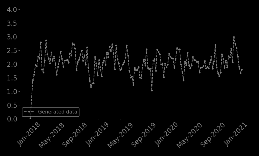
Figure 1. Generated AR process
The pattern might look like a simple random process (and in part it is), but each points (starting from 0) is calculated using the following equation:
xt = δ + φ1 xt-1 + w
Where:
δ = 1
φ1 = 0.5
and w is normally distributed with variance of σ2ε = 0.1
To be precise, this process is called AR 1 because xt is a function of itself at time t-1, φ1xt-1. Should we add the term φ2 xt-2 into the equation, the process would be called AR 2, and so forth. Feel free to change the model parameters in the section 1 of the code to simulate a different AR 1 process.
It is interesting to observe that the process increases rapidly from zero and then it fluctuates around its mean. There are specific formulas to calculate the mean and other statistics (e.g. variance) of an AR 1 process. I put some links at the end of the post. In section 2 of the code I implemented some of them and show how the theoretical values are very close to the ones calculated empirically from the generated data.
Calibration
Now let’s calibrate an AR 1 model using this data and check if we would obtain the same model coefficients we previously used to generate the data. We can divide the data in two parts: the calibration dataset (from the beginning until 2020-07-05) and testing dataset. The code of section 3 runs the calibration and plots some diagnostic plots.
As expected, the calibrated coefficients (table 1) are very close to the ones we defined. The diagnostic plots (Figure 2) do not highlight any problems in the formulation of the mathematical model. This was also expected since the data were exactly generated to mimic an AR 1 process.
Table 1: Model coefficients from calibration.
| Symbol | Coef | P > |z| |
|---|---|---|
| δ | 1.06 | 0.000 |
| φ1 | 0.48 | 0.000 |
| σ2ε | 0.10 | 0.000 |
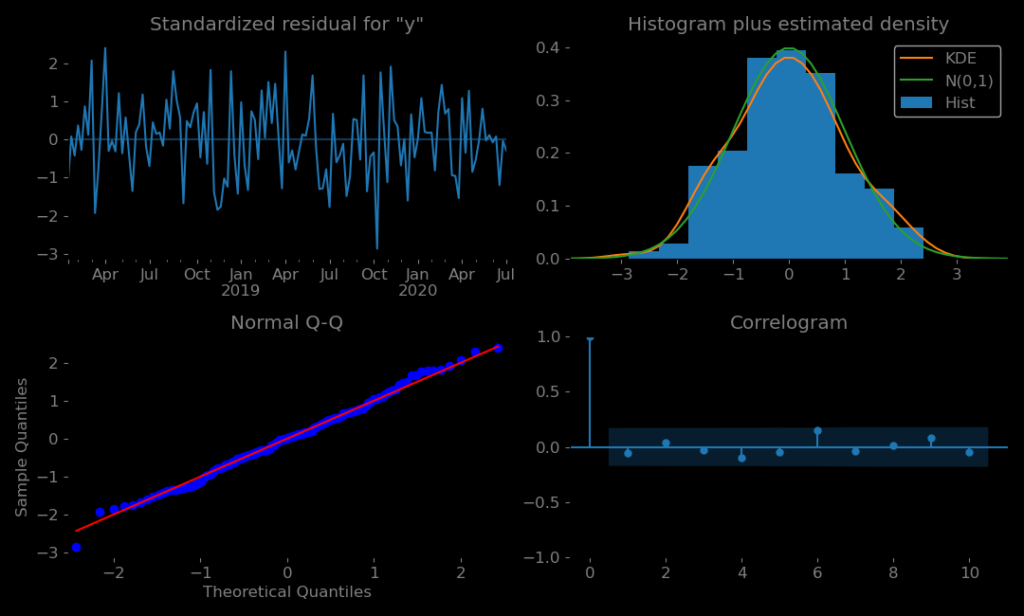
Figure 2. Diagnostic plots.
Predictions
Now let’s generate model predictions and plot model performances during the calibration and testing phase (Figure 3, section 4 of the code).
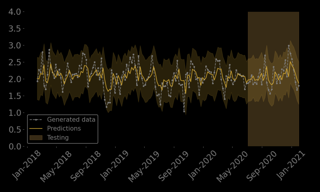
Figure 3. One-step model predictions.
As expected the model captures quite well the over trend, during both the calibration and testing phases. The fact that there is not a perfect overlap between the generated data and predictions is due to the random component (w) in the generated data.
If you noticed I set the option dynamic = False. This means a one-step prediction is implemented. If we re-run the code with dynamic = start_test (Figure 4), a recursive strategy to predict each value is implemented. This means that the prediction for the prior time step is used as an input for making a prediction on the following time step. As can be seen in the graph, after a few steps the predictions converge to the mean value of the model.
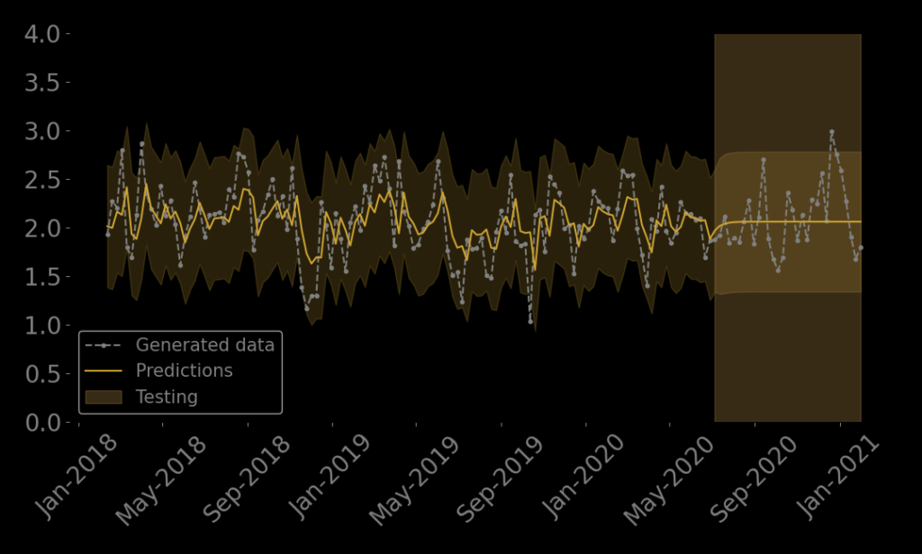
Figure 4. Recursive multi-step model predictions.
Code
#%% IMPORT LIBRARIES
import os

import numpy as np
import pandas as pd

## Import the library for plotting
import matplotlib.pyplot as plt
### It sets the graph option to default
plt.rcParams.update(plt.rcParamsDefault)

import matplotlib.dates as mdates

## Seasonal AutoRegressive Integrated Moving Average with eXogenous regressors model
from statsmodels.tsa.statespace.sarimax import SARIMAX

------------------------------------------SECTION 1-------------------------------------------------------------
#%% SIMULATE AND PLOT THE AR(1) PROCESS

## Define a range of date and frequnecy
date_index = pd.date_range(start='2018-01-01',
                           end='2021-02-01',
                           freq='W')

## Define the parameters of the AR(1) model
delta = 1 # <---------------------------CHANGE HERE
phi = 0.5  # <---------------------------CHANGE HERE
sigma2 = 0.1 # <---------------------------CHANGE HERE

## Define the structure of the AR(1) model
arima_structure = (1, 0, 0)
sarima_structure = (0, 0, 0, 0)
empty_dataset = np.zeros(len(date_index))

## Initialise the model
### Set the seed to make results replicable
np.random.seed(1)
mod = SARIMAX(empty_dataset,
              order = arima_structure,
              seasonal_order = sarima_structure,
              trend="c",
              initialization = "diffuse")

## Generate the process using the defined parameters
simulation = mod.simulate([delta, phi, sigma2],
                           len(date_index))

df = pd.Series(data = simulation,
               index = date_index)

## Make the plot
plt.plot(df,
        label = "Generated data",
        linestyle='--',
        marker='o',
        markersize = 4,
        linewidth = 2,
        color = "gray")

plt.ylim(0, 4)

## Modify the date format
date_form = mdates.DateFormatter("%b-%Y")
plt.gca().xaxis.set_major_formatter(date_form)
plt.tick_params(axis='x', labelrotation=45)

plt.legend(loc ="lower left",
           fontsize = 15)

------------------------------------------SECTION 2-------------------------------------------------------------
#%% CALCULATE THE AR(1) STATISTICS

burn_out = 5 # <----------------CHANGE HERE

## Empirically
empirical_mean = round(df[burn_out:].mean(),2)
empirical_variance = round(df[burn_out:].var(),2)
empirical_correlation_lag1 = round(df[burn_out:].corr(df[burn_out:].shift()),2)

## Theoretical
theorethical_mean = delta/(1-phi)
theoretical_variance = sigma2/(1-(phi)**2)
theoretical_correlation_lag1 = phi**(1)

------------------------------------------SECTION 3-------------------------------------------------------------
#%% CALIBRATE THE AR(1) MODEL

## Define the test and training dataset
start_train = pd.to_datetime('2018-01-01')
start_test = pd.to_datetime('2020-07-05')

df_train = df[start_train:start_test]
df_test = df[start_test:]

## Define the structure of the AR(1) model
arima_structure = (1,0,0)
sarima_structure = (0, 0, 0, 0)

## Initialise the model on the training dataset
model = SARIMAX(endog = df_train,
                exog = None,
                order = arima_structure,
                seasonal_order = sarima_structure,
                trend = "c",
                initialization = "diffuse")


## Calibrate the model
model_fit = model.fit()

## Display model summary
print(model_fit.summary())

------------------------------------------SECTION 4-------------------------------------------------------------

#%%  GENERATE MODEL PREDICTIONS

## Initialise model on the whole dataset
model = SARIMAX(endog = df[start_train:],
                exog = None,
                order = arima_structure,
                seasonal_order = sarima_structure,
                trend = "c",
                initialization = "diffuse")

## Generate model predictions using calibrated model parameters
res = model.filter(model_fit.params)
prediction = res.get_prediction(start = 0,
                                end = len(df[start_train:])-1,
                                dynamic=False) # <--------CHANGE HERE (dynamic = start_test to make dynamic)
ci = prediction.conf_int()

#%% MAKE THE PLOT

burn_out = 5 # <---------------------------CHANGE HERE

## Plot generated data
plt.plot(df[burn_out:],
           color='gray',
           linestyle='--',
           marker='o',
           markersize = 3,
           linewidth=1.5,
           label = "Generated data")


## Plot model predictions
plt.plot(prediction.predicted_mean[burn_out:],
         color=color_1,
         linewidth=1.5,
         label = "Predictions")

## Plot confidence intervals
plt.fill_between(ci.index[burn_out:],
                 ci[burn_out:][ci.columns[0]], ci[burn_out:][ci.columns[1]],
                 alpha=0.2,
                 color = color_1)

plt.axvspan(start_test,
            max(df.index),
            alpha = 0.3,
            label = "Testing",
            color = color_3)

## Modify the date format
date_form = mdates.DateFormatter("%b-%Y")
plt.gca().xaxis.set_major_formatter(date_form)
plt.tick_params(axis='x', labelrotation=45)

plt.legend(loc="lower left",
           fontsize = 15)
plt.ylim(0, 4)
References
Properties of AR model: https://online.stat.psu.edu/stat510/lesson/1/1.2